Turning your excel into abstract art generator

Yesterday, while I was doing some data analysis and got tired, then decided to do some artistic stuff with MS Excel, and I was amazed by the unintentional results.

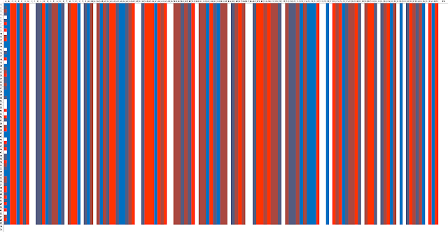Color Strip Generated with Excel

You may wonder how to do that? it is really simple, but a lot of fun. Let's get started and try it out!!!!



Preparation:
First, Prepare the canvas. Select around 100 columns and 100 rows, if you want to play in a square, shrink the cell a bit into squares.
Then, while the matrix is selected, go to Number-->Custom, like the below image, and put in ;;; in the type. This will hide the numbers and other value in the excel cell.

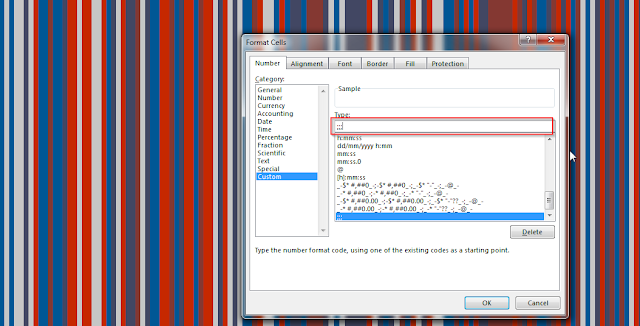Hide numbers in excel cells

Next, let's populate the formula.

For the image at the beginning, I started with row 1, put in  =RANDBETWEEN(1,5)
Simply put the formula in cellA1, and then drag to the right to fill will do, unless you want some other fancy stuff.
and drag down to fill in column 1 the same formula from cell A1, i.e. =RANDBETWEEN(1,5)
At cells(2,2) and the rest of the matrix (just drag), put in: =IF(A2<10,A2*B1,SQRT(ABS(A2)))
then select whole matrix, go to Conditioning Formatting, Color Scale, then play around with the 2-color scale or 3-color scale.

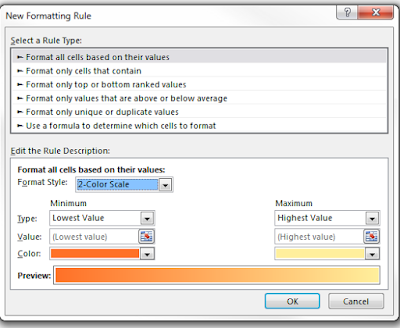Color Scales in Conditional Formatting

As you have noticed, I used the random function (Rand() or RandBetween(*,*)) to generate the start number, then I work based on that. However, in order to generate some interesting image with certain continuity, you need to capture the changes around the certain cell. Otherwise, you will get just random color noises.

Meanwhile, the color you selected from the conditioning format is as important (such as 2 vs. 3 color, and the set up of the value to lowest/highest value or a fixed number), if not more important, as the formula itself. 

Try it out, and leave a line if you have any questions, and it will be great if you have other great images to share.

The below are some other formulas I used to generate other interesting images, but the steps are the same. 

Formulas:
In row 1, put in  =RANDBETWEEN(1,5)
and put in the same in column 1, i.e. =RANDBETWEEN(1,5)
At cells(2,2) to the end of the matrix, put in: =B1
then select whole matrix, go to Conditioning Formatting, Color Scale, then play around with the 2-color scale or 3-color scale.

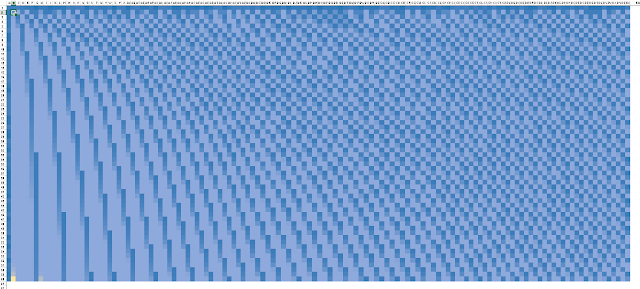Wave generated with MS Excel

Formulas:
In row 1, put in  =RANDBETWEEN(1,5)
and put in the same in column 1, i.e. =RANDBETWEEN(1,5)
At cells(2,2) to the end of the matrix, put in: =IF((A1+A2+B1)>3*A1,IF(A1*A2<100,A1*A2,SQRT(A1*A2)),(A1+A2+B1)/2)
then select whole matrix, go to Conditioning Formatting, Color Scale, then play around with the 2-color scale or 3-color scale.

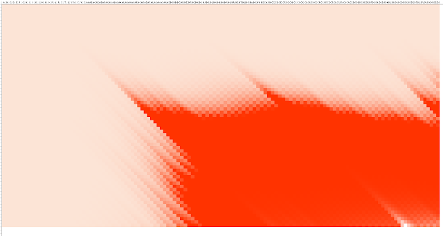Flare Generated with MS Excel

Formulas:
In row 1, put in  =RANDBETWEEN(1,5)
and put in the same in column 1, i.e. =RANDBETWEEN(1,5)
At cells(2,2) to the end of the matrix, put in: =SQRT(ABS(B1))
then select whole matrix, go to Conditioning Formatting, Color Scale, then play around with the 2-color scale or 3-color scale.

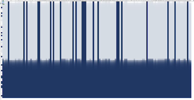Woods Generated with MS Excel

Formula:
In row 1, put in  =RANDBETWEEN(1,5)
and put in the same in column 1, i.e. =RANDBETWEEN(1,5)
At cells(2,2) to the end of the matrix, put in: =IF(A2<10,(A2+B1),SQRT(ABS(A1+B1))+B1/ABS(A1))
then select whole matrix, go to Conditioning Formatting, Color Scale, then play around with the 2-color scale or 3-color scale.

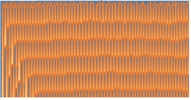The wall Generated by MS Excel

Formula:
In row 1, put in  =RANDBETWEEN(1,5)
and put in the same in column 1, i.e. =RANDBETWEEN(1,5)
At cells(2,2) to the end of the matrix, put in: =SUM(A1:$EA$1)/(B1+A1)
then select whole matrix, go to Conditioning Formatting, Color Scale, then play around with the 2-color scale or 3-color scale.

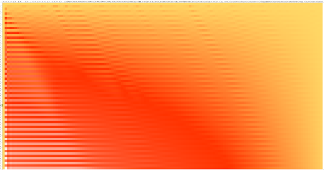Dancing Flag Generated by MS Excel